Default or No Default?

In this post, I will briefly go over an example of a Scikit-learn-based implementation of a support vector machine–a popular example of a supervised learning model. The code blocks below came from one of StatQuest’s public-domain tutorials on support vector machines, but the line-by-line explanations of the code are in my own words. As usual, the data used in this exercise came from the publicly available UCI Machine Learning Repository.

Importing Packages & Data

First, we need to import all the necessary libraries/packages/modules, including pandas, numpy, matplotlib, and etc.

import pandas as pd
import numpy as np
import matplotlib.pyplot as plt
import matplotlib.colors as colors
from sklearn.utils import resample
from sklearn.model_selection import train_test_split
from sklearn.preprocessing import scale
from sklearn.svm import SVC
from sklearn.model_selection import GridSearchCV
from sklearn.metrics import confusion_matrix
from sklearn.metrics import plot_confusion_matrix
from sklearn.decomposition import PCA

df = pd.read_excel('dccc.xlsx', header=1)

Here, we read the excel file we need–“dccc.xlsx”–that I downloaded from the repository. “DCCC” stands for the name of the data–“default of credit card users.”

df.head()

	ID	LIMIT_BAL	SEX	EDUCATION	MARRIAGE	AGE	PAY_0	PAY_2	PAY_3	PAY_4	...	BILL_AMT4	BILL_AMT5	BILL_AMT6	PAY_AMT1	PAY_AMT2	PAY_AMT3	PAY_AMT4	PAY_AMT5	PAY_AMT6	default payment next month
0	1	20000	2	2	1	24	2	2	-1	-1	...	0	0	0	0	689	0	0	0	0	1
1	2	120000	2	2	2	26	-1	2	0	0	...	3272	3455	3261	0	1000	1000	1000	0	2000	1
2	3	90000	2	2	2	34	0	0	0	0	...	14331	14948	15549	1518	1500	1000	1000	1000	5000	0
3	4	50000	2	2	1	37	0	0	0	0	...	28314	28959	29547	2000	2019	1200	1100	1069	1000	0
4	5	50000	1	2	1	57	-1	0	-1	0	...	20940	19146	19131	2000	36681	10000	9000	689	679	0

5 rows × 25 columns

Here, the columns that read “PAY_AMT” indicate how much was paid over the past six months, with the number following PAY_AMT indicating the month. The numbers in the column for education indicate the level of education that one received. The limit balance tells us how much is left in each person’s balance. Finally, default payment next month is the variable that we wish to predict. The following is a brief summary of the meaning of the values.

• Default
  • 0: Did not default
  • 1: Defaulted
• Pay
  • -1: Bill paid on time
  • 1: Bill paid one month late
  • n: Bill paid n months late

df.rename({'default payment next month' : 'Default'}, axis = 'columns', inplace=True)
df.head() 

	ID	LIMIT_BAL	SEX	EDUCATION	MARRIAGE	AGE	PAY_0	PAY_2	PAY_3	PAY_4	...	BILL_AMT4	BILL_AMT5	BILL_AMT6	PAY_AMT1	PAY_AMT2	PAY_AMT3	PAY_AMT4	PAY_AMT5	PAY_AMT6	Default
0	1	20000	2	2	1	24	2	2	-1	-1	...	0	0	0	0	689	0	0	0	0	1
1	2	120000	2	2	2	26	-1	2	0	0	...	3272	3455	3261	0	1000	1000	1000	0	2000	1
2	3	90000	2	2	2	34	0	0	0	0	...	14331	14948	15549	1518	1500	1000	1000	1000	5000	0
3	4	50000	2	2	1	37	0	0	0	0	...	28314	28959	29547	2000	2019	1200	1100	1069	1000	0
4	5	50000	1	2	1	57	-1	0	-1	0	...	20940	19146	19131	2000	36681	10000	9000	689	679	0

5 rows × 25 columns

Here, I changed the name of the last column from “default payment next month” to simply “default.” To do that, I specified the name of the column before and after the change within curly braces. The axis='columns'indicates that I wish to change a column name, and inplace=True shows that I am changing the original dataframe object, not a copy of it.

df.drop('ID', axis=1, inplace=True) # axis=1 parameter for df.drop() indicates a removal of a column.  
df.head()

	LIMIT_BAL	SEX	EDUCATION	MARRIAGE	AGE	PAY_0	PAY_2	PAY_3	PAY_4	PAY_5	...	BILL_AMT4	BILL_AMT5	BILL_AMT6	PAY_AMT1	PAY_AMT2	PAY_AMT3	PAY_AMT4	PAY_AMT5	PAY_AMT6	Default
0	20000	2	2	1	24	2	2	-1	-1	-2	...	0	0	0	0	689	0	0	0	0	1
1	120000	2	2	2	26	-1	2	0	0	0	...	3272	3455	3261	0	1000	1000	1000	0	2000	1
2	90000	2	2	2	34	0	0	0	0	0	...	14331	14948	15549	1518	1500	1000	1000	1000	5000	0
3	50000	2	2	1	37	0	0	0	0	0	...	28314	28959	29547	2000	2019	1200	1100	1069	1000	0
4	50000	1	2	1	57	-1	0	-1	0	0	...	20940	19146	19131	2000	36681	10000	9000	689	679	0

5 rows × 24 columns

Preprocessing the Data

As with any type of data analysis, the collected data must be preprocessed, and any missing values either need to be found manually, or substituted in via an educated guess.

Checking type of data for category

Before we analyze the data, we need to make sure that a single column’s data type is uniform for all columns. We do that calling df.dtypes, which presents us with a list of the data type for all twenty-four columns.

df.dtypes 

LIMIT_BAL    int64
SEX          int64
EDUCATION    int64
MARRIAGE     int64
AGE          int64
PAY_0        int64
PAY_2        int64
PAY_3        int64
PAY_4        int64
PAY_5        int64
PAY_6        int64
BILL_AMT1    int64
BILL_AMT2    int64
BILL_AMT3    int64
BILL_AMT4    int64
BILL_AMT5    int64
BILL_AMT6    int64
PAY_AMT1     int64
PAY_AMT2     int64
PAY_AMT3     int64
PAY_AMT4     int64
PAY_AMT5     int64
PAY_AMT6     int64
Default      int64
dtype: object

df.dtypes shows the uniformity of the data within each column, which tells us two things.

1. There are no ‘mixed’ values consisting of letters and numbers.

2. There are no string-type placeholder values for missing data, or ‘NA values.’

Unfortunately, when we look at the unique numerical values, we see that zero was used as a placeholder value for missing data. Therefore, we will need to either “impute,” or calculate, the value for the placeholder zero, or remove the rows containing the zero. Since the process of cross validation, which we will use later to determine gamma and C (two parameters of SVM models), performs best when there aren’t too many rows, we will remove the 68 rows that contain missing values.

df['EDUCATION'].unique()

array([2, 1, 3, 5, 4, 6, 0], dtype=int64)

df.loc[(df['EDUCATION'] == 0) | (df['MARRIAGE'] == 0)]

	LIMIT_BAL	SEX	EDUCATION	MARRIAGE	AGE	PAY_0	PAY_2	PAY_3	PAY_4	PAY_5	...	BILL_AMT4	BILL_AMT5	BILL_AMT6	PAY_AMT1	PAY_AMT2	PAY_AMT3	PAY_AMT4	PAY_AMT5	PAY_AMT6	Default
218	110000	2	3	0	31	0	0	0	0	0	...	73315	63818	63208	4000	5000	3000	3000	3000	8954	0
809	160000	2	2	0	37	0	0	0	0	0	...	28574	27268	28021	35888	1325	891	1000	1098	426	0
820	200000	2	3	0	51	-1	-1	-1	-1	0	...	780	390	390	0	390	780	0	390	390	0
1019	180000	2	3	0	45	-1	-1	-2	-2	-2	...	0	0	0	0	0	0	0	0	0	0
1443	200000	1	3	0	51	-1	-1	-1	-1	0	...	2529	1036	4430	5020	9236	2529	0	4430	6398	0
...	...	...	...	...	...	...	...	...	...	...	...	...	...	...	...	...	...	...	...	...	...
28602	200000	2	3	0	37	1	-1	-1	-1	-1	...	4000	22800	5716	35000	5000	4000	22800	5716	0	0
28603	110000	2	3	0	44	2	2	2	2	2	...	41476	42090	43059	2000	2000	1700	1600	1800	1800	1
28766	80000	2	3	0	40	2	2	3	2	-1	...	1375	779	5889	5000	0	0	885	5889	4239	0
29078	100000	2	3	0	56	1	2	0	0	2	...	31134	30444	32460	0	1500	2700	0	2400	0	0
29111	300000	2	3	0	53	-2	-2	-2	-2	-2	...	0	0	0	0	0	0	0	0	0	0

68 rows × 24 columns

len(df.loc[(df['EDUCATION'] == 0) | (df['MARRIAGE'] == 0)])

68

Here, based on the fact that the zero values in either the education or the marriage columns imply missing values, we will remove the rows containing the zeros. In fact, as shown above, there are a total of 68 rows that contain zero for either the education or the marriage columns. These rows will be removed, and then the data will be trimmed to a 1,000 rows, since support vector machines work best for moderate sized datasets.

Removal of rows containing missing data & Trimming of the dataset

To create a new dataset containing less numbers of rows and no zeros for missing values, we will create a new dataframe object called df_no_missing

df_no_missing = df.loc[(df['EDUCATION'] != 0) & (df['MARRIAGE'] != 0)]

print('length of new dataframe : ', len(df_no_missing))
print(df_no_missing['EDUCATION'].unique())
print(df_no_missing['MARRIAGE'].unique())

length of new dataframe :  29932
[2 1 3 5 4 6]
[1 2 3]

.unique() shows the unique values within the column. As we can see, there are no zeros in any of the two columns, ‘education’ and ‘marriage.’

Support vector machine requires optimization for the right value of parameter X, which in turn necessitates a process called ‘cross validation.’ Unfortunately, cross validation works efficiently with relatively moderate sized datasets, so we need to downsample the size of the dataset to a 1,000.

Here, we split the default column into two different dataframe objects–one containing zero’s and the other containing one’s.

df_no_default = df_no_missing[df_no_missing['Default'] == 0]
df_default = df_no_missing[df_no_missing['Default'] == 1]

Then we resample from the pool of around 30,000 rows to select 1,000 rows. The resample method takes replace=False to mean that the selection pool is not refilled with already selected choices, and n_samples=1000 specifies the number of rows (samples) to select.

df_no_default_downsampled = resample(df_default, replace=False, n_samples=1000, random_state=42)
df_default_downsampled = resample(df_no_default, replace=False, n_samples=1000, random_state=42)

Then we join the two samples together to make a joint dataframe object of 2,000 rows that were selected via resample().

df_downsample = pd.concat([df_no_default_downsampled, df_default_downsampled])
len(df_downsample)

2000

One-Hot Encoding: Changing categorical data to columns of binary values

Above, the category corresponding to marriage contained numbers 1, 2, and 3. If we take these counts to be continuous, then the support vector machine is more likely to view people with closer numbers–say, 2 and 3–as similar when creating the decision boundary.

However, since the integers in that category are categorical, two people with values closer together (2,3) are equally likely to be similar to each other (in terms of default status), than pairs with values not closer together, such as (1,2).

Due to this problem, we need to convert the column containing 1’s, 2’s, and 3’s for marital status into three separate columns, containing only 0’s and 1’s.

X = df_downsample.drop('Default', axis=1).copy()
y = df_downsample['Default'].copy()

pd.get_dummies(X, columns=['MARRIAGE']).head()

	LIMIT_BAL	SEX	EDUCATION	AGE	PAY_0	PAY_2	PAY_3	PAY_4	PAY_5	PAY_6	...	BILL_AMT6	PAY_AMT1	PAY_AMT2	PAY_AMT3	PAY_AMT4	PAY_AMT5	PAY_AMT6	MARRIAGE_1	MARRIAGE_2	MARRIAGE_3
19982	300000	2	1	47	3	2	2	2	2	2	...	5000	0	0	0	0	0	0	1	0	0
19350	80000	2	2	36	2	0	0	-2	-2	-2	...	0	1700	0	0	0	0	0	0	1	0
17057	30000	2	3	22	2	2	0	0	0	0	...	11711	0	1687	1147	524	400	666	0	1	0
26996	80000	1	1	34	2	2	2	2	2	2	...	67007	2800	3000	2500	2600	2600	2600	0	1	0
23621	210000	2	3	44	-2	-2	-2	-2	-2	-2	...	14793	13462	17706	0	5646	14793	7376	1	0	0

5 rows × 25 columns

X_encoded = pd.get_dummies(X, columns=['SEX', 'EDUCATION', 'MARRIAGE', 'PAY_0', 'PAY_2', 'PAY_3', 'PAY_4', 'PAY_5', 'PAY_6'])
X_encoded.head()

	LIMIT_BAL	AGE	BILL_AMT1	BILL_AMT2	BILL_AMT3	BILL_AMT4	BILL_AMT5	BILL_AMT6	PAY_AMT1	PAY_AMT2	...	PAY_5_7	PAY_6_-2	PAY_6_-1	PAY_6_0	PAY_6_2	PAY_6_3	PAY_6_4	PAY_6_5	PAY_6_6	PAY_6_7
19982	300000	47	5000	5000	5000	5000	5000	5000	0	0	...	0	0	0	0	1	0	0	0	0	0
19350	80000	36	19671	20650	0	0	0	0	1700	0	...	0	1	0	0	0	0	0	0	0	0
17057	30000	22	29793	29008	29047	29507	11609	11711	0	1687	...	0	0	0	1	0	0	0	0	0	0
26996	80000	34	61231	62423	63827	64682	65614	67007	2800	3000	...	0	0	0	0	1	0	0	0	0	0
23621	210000	44	11771	13462	17706	0	5646	14793	13462	17706	...	0	1	0	0	0	0	0	0	0	0

5 rows × 81 columns

Scaling the data for using the radial basis function in SVM

To use the radial basis function as the kernel function in the SVM module of Scikit-learn (kernal=rbf), the data in those 81 columns need to be scaled to have mean=0 and std=1. We will scale the data using the scale() function.

By using train_test_split, we will split up the data in the X_encoded and y objects into training data (75% of total data in X_encoded and y) and testing data (25% of total data in X_encoded and y).

X_train, X_test, y_train, y_test = train_test_split(X_encoded, y, random_state=42)
X_train_scaled  = scale(X_train)
X_test_scaled = scale(X_test)

Creating and interpreting the SVM model

Using GridSearchCV to find C and gamma

To optimize the regularization constant C (higher C means choosing lower margins between hyperplane and data points for accuracy improvement), gamma (higher gamma means prioritizing points closer to the hyperplane), we will use a GridSearchCV object called optimal_params. For the kernel function, the GridSearchCV object could suggest other possible kernel functions aside from rbf (observe the cv=5, the cross validation fold number parameter), but for simplicity, we will use rbf.

param_grid = [{'C': [0.5, 1, 10, 100], 'gamma': ['scale', 1, 0.1, 0.01, 0.001, 0.0001], 'kernel': ['rbf']}]

optimal_params = GridSearchCV(SVC(), param_grid, cv=5, scoring='accuracy', verbose=0)

optimal_params.fit(X_train_scaled, y_train)
print(optimal_params.best_params_)

{'C': 100, 'gamma': 0.001, 'kernel': 'rbf'}

Creating and interpreting the SVM model

Here, we will create an SVM object by specifying the C (regularization constant) as 100, and gamma as 0.001. Then we must “train” the object, or allow it to find the optimum parameters for constructing the decision boundary. We will use .fit() to accomplish the task.

shell_of_SVM = SVC(random_state=42, C=100, gamma=0.001)
shell_of_SVM.fit(X_train_scaled, y_train) # "training the SVM", or finding the optimum parameters for the SVM decision boundary

plot_confusion_matrix(shell_of_SVM, X_test_scaled, y_test, values_format='d', display_labels = ["No Default", "Defaulted"])

<sklearn.metrics._plot.confusion_matrix.ConfusionMatrixDisplay at 0x1f826a77970>

Confusion Matrix with Scikit-learn

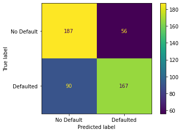
Here is the result, which shows that 187 people out of the 243 that did not default were correctly predicted to have not defaulted, For the 237 people that did default, 167 people were correctly predicted to have defaulted.

---

Conclusion

In this post, I explained how to implement a support vector machine model using Scikit-learn, referencing one of StatQuest’s tutorials on support vector machines. Even though the actual SVC() object did not come until the very end, I believe that speaks to the difficulty and importance of preprocessing the data, which actually took up the bulk of the work. As for optimizing the parameters of the SVC model, I used cross-validation using GridSearchCV function, and furthermore, I used rbf (radial basis function) for the kernel. As for the latter, I do not yet fully understand its complete mathematical basis, but in the future, I hope that I can to the fullest extent. I hope you enjoyed reading this post.