
Logistic Regression
In this post, I will go over the “hello world” of machine learning–logistic regression. This post references Andrew Ng’s 2020 lecture on machine learning, available on Youtube’s StanfordOnline channel.
Linear Regression
Before learning about logistic regression, a basic understanding of linear regression would be helpful. Linear regression, as the name implies, is an actual regression algorithm, unlike logistic regression, which is actually a classifier. The goal of linear regression is to predict values for a continuous dependent variable using the samples’ features.
To illustrate, suppose that there are $m$ samples of houses and that each sample has $n$ features. For example, we could have three samples of houses with two features each–the area and the number of bedrooms. Based on the feature values, our goal is to predict the prices of houses. We will denote the sample number by the superscript index in parentheses, and the feature number by the subscript index.
| Area | Bedrooms | Price |
|---|---|---|
| $x_1^{(1)}$ | $x_2^{(1)}$ | $y^{(1)}$ |
| $x_1^{(2)}$ | $x_2^{(2)}$ | $y^{(2)}$ |
In predicting the houses’ prices, we could set up a linear model with weights $\theta_0$, $\theta_1$, and $\theta_2$ as coefficients to feature values $x_1$ and $x_2$.
\[h_\theta(\vec{x}) := \theta_0 + \theta_1x_1 + \theta_2x_2\] \[\theta = \begin{bmatrix} \theta_0 \\ \theta_1 \\ \theta_2 \end{bmatrix} \;\;\;\;\;\;\; \vec{x} = \begin{bmatrix} 1 \\ x_1 \\ x_2 \end{bmatrix}\]The result–the price of the house–can be noted as $h_\theta(\vec{x})$, and would be equal to the linear combination of the elements of the coefficient and feature vectors. Alternatively, we could use the dot product notation between the vectors.
\[h_\theta(\vec{x}) := \sum_{i = 0}^{n} \theta_i \cdot x_i = \theta^\top \cdot \vec{x}\] \[[\theta_0, \theta_1, \theta_2] \cdot \begin{bmatrix} x_0 \\ x_1 \\ x_2 \end{bmatrix} = \theta_0x_0 + \theta_1x_1 + \theta_2x_2 \;\;\;\;\;\;\; \text{(for $x_0 = 1$)}\]As stated above, the goal of linear regression is to find a way to best predict values for a continuous variable. Another way to state this goal is to find weight parameters $\theta_0$ … $\theta_n$ that minimize the least-squares cost function, given some training samples. To find these weight parameters, one can perform gradient descent on the least-squares cost function that takes weight parameters as variables.
Gradient Descent & Weight Update
One-sample cost function
Now extend the housing price illustration to include $m$ samples of houses with $n$ features each. Then we would have a table that looks like the following.
| Area ($\theta_1$) | Bedrooms ($\theta_2$) | Bathrooms ($\theta_3$) | … | Fireplace ($\theta_n$) | Price |
|---|---|---|---|---|---|
| $x_1^{(1)}$ | $x_2^{(1)}$ | $x_3^{(1)}$ | … | $x_n^{(1)}$ | $y^{(1)}$ |
| $x_1^{(2)}$ | $x_2^{(2)}$ | $x_3^{(2)}$ | … | $x_n^{(2)}$ | $y^{(2)}$ |
| $x_1^{(3)}$ | $x_2^{(3)}$ | $x_3^{(3)}$ | … | $x_n^{(3)}$ | $y^{(3)}$ |
| … | … | … | … | … | … |
| $x_1^{(m)}$ | $x_2^{(m)}$ | $x_3^{(m)}$ | … | $x_n^{(m)}$ | $y^{(m)}$ |
For the case of the one-sample cost function, take the first row (or first sample) of the table.
| Area ($\theta_1$) | Bedrooms ($\theta_2$) | Bathrooms ($\theta_3$) | … | Fireplace ($\theta_n$) | Price |
|---|---|---|---|---|---|
| $x_1^{(1)}$ | $x_2^{(1)}$ | $x_3^{(1)}$ | … | $x_n^{(1)}$ | $y^{(1)}$ |
Next, we define the cost function, $J(\vec{\theta})$, for that single row only. For vector $\vec{x}^{(1)} = \big[x_1^{(1)}, x_1^{(2)}, x_1^{(3)} … x_1^{(n)}\big]$, the cost function $J(\vec{\theta})$ takes the following form.
\[J(\vec{\theta}) = \frac{1}{2} \cdot (h_\theta (\vec{x}^{(1)}) - y^{(1)})^2\] \[= \frac{1}{2} \cdot (\sum_{k=0}^{n}\theta_k x^{(1)}_k - y^{(1)})^2\] \[= \frac{1}{2} \cdot (\theta_0 x^{(1)}_0 + \theta_1 x^{(1)}_1 + ... + \theta_n x^{(1)}_n - y^{(1)})^2\]Then for that one sample, the derivative of the cost function with respect to $\theta_j$ is:
\[J_{\theta_j} = \big[\sum_{k=0}^{n}\theta_k x^{(1)}_k - y^{(1)}\big] \cdot \frac{\partial}{\partial\theta_j}\big[\sum_{k=0}^{n}\theta_k x^{(1)}_k - y^{(1)}\big]\] \[= \big[\sum_{k=0}^{n}\theta_k x^{(1)}_k - y^{(1)}\big] \cdot x^{(1)}_j\]More-than-one-sample cost function
For tables with $m$ samples, or rows, the cost function would be in the following form. Note that in this summation, we are no longer summing with respect to the weight parameter indices, but with respect to the samples.
\[J(\theta) = \frac{1}{2} \cdot \sum_{i=1}^{m} (h_\theta(x^{(i)}) - y^{(i)})^2\]where
\[h_\theta(\vec{x}^{(i)}) = \theta_1x_1^{(i)} + \theta_2x_2^{(i)} + ... + \theta_nx_n^{(i)}\]LMS Update Rule
The purpose of gradient descent is to essentially find weight parameters that minimize the loss function, when provided with sample data. One way to do gradient descent is to start with random values for the weight parameters, and then constantly update those parameters in the direction that we need. One of the methods for updating the parameter values is called the “LMS update rule,” or the “Least-Mean-Square update rule.”
The LMS update rule can be stated by the following equality.
\[\theta_j := \theta_j - \alpha \cdot [\frac{\partial}{\partial\theta_j} J(\theta)] \;\;\;\;\text{for $\alpha > 0$}\]That is, for learning rate $\alpha$, we wish to update $\theta_j$ –the $j^{th}$ weight parameter– by $\alpha$ multiplied by the gradient of the cost function with respect to the $j^{th}$ weight parameter. Consider the fact that we defined the cost function $J(\theta)$ as the following expression for the case of more than one sample.
\[J(\theta) = \frac{1}{2} \cdot \sum_{i=1}^{m} (h_\theta(x^{(i)}) - y^{(i)})^2\]Now look at the expression inside the summation.
\[\frac{1}{2} \big(h_\theta(\vec{x}^{(i)})-y^{(i)}\big)^{2} \;\;\; \text{for} \;\;\;h_\theta(\vec{x}^{(i)}) = \theta_1x_1^{(i)} + \theta_nx_n^{(i)} + ... + \theta_nx_n^{(i)}\]Partially differentiating this expression with respect to $\theta_j$ would get us the following result:
\[\frac{\partial}{\partial\theta_j} \big[\frac{1}{2} \{h_\theta(\vec{x}^{(i)})-y^{(i)}\}^{2}\big] = \big[h_\theta(\vec{x}^{(i)})-y^{(i)}\big] \cdot x_j^{(i)} \;\;\;\;\;\;\;\;\; \tag{1}\]Therefore, going back to the LMS update rule above, we see that the expression inside the brackets can be put as the followng:
\[[\frac{\partial}{\partial\theta_j} J(\theta)] = \frac{\partial}{\partial\theta_j} \big[ \frac{1}{2} \sum_{i=1}^{m} (h_\theta(x^{(i)}) - y^{(i)})^2 \big]\]Since partial differentiating after the summation is the same as summing the already partially differentiated terms, we can simplify the above expression as the following one.
\[= \sum_{i=1}^{m} \frac{\partial}{\partial\theta_j} \big[ \frac{1}{2} (h_\theta(x^{(i)}) - y^{(i)})^2 \big]\]And the expression inside the summation is simply what we previously got with the equation labeled as (1).
Therefore,
\[= \sum_{i=1}^{m} \big[h_\theta(\vec{x}^{(i)})-y^{(i)}\big] \cdot x_j^{(i)}\]Now, we can rewrite the LMS update rule stated above,
\[\theta_j := \theta_j - \alpha \cdot [\frac{\partial}{\partial\theta_j} J(\theta)] \;\;\;\;\text{for $\alpha > 0$}\]as the following:
\[\theta_j := \theta_j - \alpha \cdot [\sum_{i=1}^{m} \{h_\theta(\vec{x}^{(i)})-y^{(i)}\} \cdot x_j^{(i)}] \;\;\;\;\text{for $\alpha > 0$}\]This expression is the LMS update rule for batch gradient descent, where we look at every sample (row) to update the weight parameter (column), once.
For stochastic gradient descent, we simply remove the summation sign from the above equation and choose a random sample $x^{(i)}$ to update the parameter $\theta_j$.
\[\theta_j := \theta_j - \alpha(h_\theta(x^{(i)})- y^{(i)})x_j^{(i)}\]Logistic Regression
Now that we have briefly looked at linear regression, let’s take a look at logistic regression.
Logistic regression is a type of classifier, and not a regression algorithm. This is because logistic regression plugs in the dot product between weight and sample vectors into a special function called the logistic (or sigmoid) function, shown below.
\[y = \frac{1}{1+e^{-x}}\]The output of this logistic function is always between zero and one, ensuring that this output can be interpreted as the probability of a certain sample belonging to a particular class. The logistic function’s simple graph is as follows.
import matplotlib.pyplot as plt
import numpy as np
import math

x = np.linspace(-5, 5, 1000)
y = 1 / (1 + np.e**(-x))

# normal: y = 1 / (sigma * np.sqrt(2*np.pi)) * np.e**(-0.5*((x-mu)/sigma)**2)

fig, ax = plt.subplots()
ax.plot(x,y)
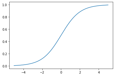
For $g(x)$ defined as the logistic (or sigmoid) function, we define $h_\theta(\vec{x})$ as the logistic function with $\theta^\top \cdot \vec{x}$ as the input value. Here, we note that $h_\theta(\vec{x})$ is $g(\theta^\top \cdot \vec{x})$, whereas in linear regression, $h_\theta(\vec{x})$ was simply $\theta^\top \cdot \vec{x}$.
\[h_\theta(\vec{x}) = g(\theta^\top \cdot \vec{x}) = \frac{1}{1+e^{-\theta^\top\vec{x}}}\]Now, given a list of vectors $\vec{x}^{(1)}$, $\vec{x}^{(2)} … \vec{x}^{(m)}$, define $X$ as the design matrix containing the list of vectors in its rows. Then the likelihood of seeing $\vec{y}$ as the target value vector when given $X$ and weight parameter vector $\vec{\theta}$ can be expressed in the following form.
\[L(\vec{\theta}) = P(\vec{y}|X ;\theta)\]If we assume that the training examples and their target values are independent from each other, the likelihood of seeing $\vec{y}$ for $\vec{x}^{(1)}$, $\vec{x}^{(2)}$ … $\vec{x}^{(m)}$ is the product of individual likelihoods. That is,
\[L(\vec{\theta}) = P(\vec{y} \;|\; X;\theta) = \prod_{i=1}^{m} p(y^{(i)} \;|\; \vec{x}^{(i)};\vec{\theta})\]When computing this likelihood, the product of individual probabilities is often too small for computers to calculate accurately, leading to underflow. This is why we normally calculate the log of the likelihood, or $log\; L(\vec{\theta})$. If we denote this value as $l(\vec{\theta})$, then $l(\vec{\theta}) := log\; L(\vec{\theta})$.
Next, we wish to update weight parameters too for logistic regression. Unlike linear regression, we update based on the likelihood function, not the cost function, because what we wish to get at the end is a likelihood or a probability, not a value.
In linear regression, we tried to find the global minimum of the cost function (a function of weight parameters) based on the training sample vectors. In other words, we updated the weight parameters in a way that minimized the cost function. That is why we followed down the gradient in gradient descent. That is, we tried to “fall in a hole” in a topological sense.
In logistic regression, however, we are trying to find the global maximum of the likelihood function (a function of weight parameters) based on training sample vectors. This is why we must update the weights in a direction that maximizes the likelihood function. In that sense, we perform gradient ascent, and that explains the $+\alpha$ in front of the $[\frac{\partial}{\partial\theta_j} l(\theta)]$.
\[\theta_j := \theta_j + \alpha \cdot [\frac{\partial}{\partial\theta_j} l(\theta)] \;\;\;\;\text{for $\alpha > 0$}\]Since $l(\theta) = log \; L(\theta)$, simply substitute the expression for $L(\theta)$ to arrive at the following result.
\[l(\theta) = log \; L(\theta) = log \; \prod_{i=1}^{m} p(y^{(i)} \;|\; \vec{x}^{(i)};\vec{\theta})\]Since we defined $h_\theta(\vec{x})$ as the probability that we would see $y = 1$ as the label if given sample vector $\vec{x}$ (and hence logistic regression), we can rewrite the following expression into a different form.
\[p(y^{(i)} \;|\; \vec{x}^{(i)};\vec{\theta}) = (h_\theta(\vec{x}))^{y^{(i)}} (1-h_\theta(\vec{x}))^{1-y^{(i)}}\]Plug this expression inside the product notation, and derive with respect to $ \theta_j$ to get $[\frac{\partial}{\partial\theta_j} l(\theta)]$. We can then use the resulting expression to find the update rule for logistic regression. The complete list of steps in terms of the math is too extensive to belong within this blog post, but the point here is that logistic regression’s weight update rule takes a similar form to that of linear regression. For more detailed explanation of the steps involved, professor Andrew Ng’s CS229 notes contain a step-by-step guide that walks the reader through the math.
Logistic Regression
In this demonstration, we will use the breast cancer dataset from the UCI ML repository, which is available in the form of a toy dataset provided by scikit-learn. After saving the data in an sklearn.utils.Bunch object called cancerData, we can visualize the dataset using pandas.DataFrame, which has been done below. The breast cancer dataset contains 569 samples, with each sample consisting of values spread across thirty columns. The columns are breast-cancer related characteristics, such as the mean radius of the cancer cells’ nuclei. The labels are zero for malignant cancer cells and one for benign cancer cells.
from sklearn.datasets import load_breast_cancer
cancerData = load_breast_cancer()
# type(cancerData) // sklearn.utils.Bunch
import pandas as pd


columnList = ["radius","texture", "perimeter","area","smoothness","compactness","concavity","concave points","symmetry","fractal dimension","radius (std error)","texture (std error)", "perimeter (std error)","area (std error)","smoothness (std error)","compactness (std error)","concavity (std error)","concave points (std error)","symmetry (std error)","fractal dimension (std error)","radius (worst)","texture (worst)", "perimeter (worst)","area (worst)","smoothness (worst)","compactness (worst)","concavity (worst)",
"concave points (worst)","symmetry (worst)","fractal dimension (worst)","result"]


# print(cancerData.data)
# print(type(cancerData.data)) # np.ndarray
# print(cancerData.target)

cancerListData = cancerData.data.tolist()
cancerListTarget = cancerData.target.tolist()


dfList = []
for i in range(len(cancerListData)):
  temp = cancerListData[i]
  temp.append(cancerListTarget[i])
  dfList.append(temp)
# print(dfList)

df = pd.DataFrame(dfList, columns = columnList)
print(df)
     radius  texture  ...  fractal dimension (worst)  result
0     17.99    10.38  ...                    0.11890       0
1     20.57    17.77  ...                    0.08902       0
2     19.69    21.25  ...                    0.08758       0
3     11.42    20.38  ...                    0.17300       0
4     20.29    14.34  ...                    0.07678       0
..      ...      ...  ...                        ...     ...
564   21.56    22.39  ...                    0.07115       0
565   20.13    28.25  ...                    0.06637       0
566   16.60    28.08  ...                    0.07820       0
567   20.60    29.33  ...                    0.12400       0
568    7.76    24.54  ...                    0.07039       1

[569 rows x 31 columns]
After splitting the data into training and testing sets using train_test_split(), we use sklearn.linear_model.LogisticRegression() to create a logistic regression object called logreg. Then we call .fit() to optimize the model parameters of logreg. and .predict() on the testing set to see how well the model performs.
from sklearn.model_selection import train_test_split

x_train, x_test, y_train, y_test = train_test_split(cancerData.data, cancerData.target, test_size=0.5)
from sklearn.linear_model import LogisticRegression

# all parameters not specified are set to their defaults
logreg = LogisticRegression()
logreg.fit(x_train, y_train)
predictions = logreg.predict(x_test)
# display(predictions)
# display(y_test)
# display(y_test.size)

count = 0
for pair in zip(predictions, y_test):
  if pair[0] != pair[1]:
    count += 1

print("Accuracy: ", len(y_test)-count, " out of ", len(y_test), " correct,", 100*(len(y_test)-count) / len(y_test), "%", "\n")

index = 0
for pair in zip(predictions, y_test):
  index += 1
  if pair[0] != pair[1]:
    print(pair, "index = ", index)
Accuracy:  273  out of  285  correct, 95.78947368421052 %

(1, 0) index =  59
(1, 0) index =  66
(0, 1) index =  76
(1, 0) index =  96
(0, 1) index =  135
(1, 0) index =  149
(0, 1) index =  162
(1, 0) index =  175
(1, 0) index =  194
(1, 0) index =  259
(0, 1) index =  273
(0, 1) index =  279
As can be seen above, the logistic regression model made with scikit-learn’s LogisticRegression() has achieved 95.7% accuracy in predicting whether test samples are malignant cancer cells or not. We also see that the model incorrectly classified samples for indexes 59, 66, 76, and etc.