Dive into Distributions

7 minute read

In this post, let’s dive into distributions.

MotivationPermalink

When studying machine learning, one undoubtedly encounters many diverse distributions. For myself, I learned about normal, binomial, Bernoulli, and $\chi^2$ distributions in high school AP Statistics, but I happened to recently come across some unfamiliar ones. In fact, after getting tired of individually looking up the distributions each time I ran into them, I decided to create my own distributions reference sheet based on what I studied.

This blog post was originally intended to contain information on seven different types of distributions. Due to the sheer length of the intended post though, I chose to first deal with the three that I saw the most frequently, but never grasped thoroughly: Bernoulli, Poisson, and Gamma distributions. For the latter two, I took notes on the derivation processes for the mean and variance using the moment generating function. The following contents are my own explanations of what I learned from one of MIT OpenCourseWare’s courses.

Bernouille Trials, DistributionPermalink

A Bernouille trial is a trial in which the only outcomes are either success or failure. When repeating Bernouilli trials, the probability of success should remain the same. When we set $X$ to be the random variable for a Bernouilli trial, we usually denote $X=1$ and $X=0$ to be the case for success and failure, respectively. If we define the probabilities for failure and success to be $P(X=0) = 1-p$ and $P(X=1) = p$ , we can combine those two expressions into a single form:

$p(x) = p^x \cdot (1-p)^{1-x}, \text{ for } x = 0,1$

In this case, it is easy to see that $p(0) = 1-p$ and $p(1) = p$ . Therefore, the expectation value $E(X)$ is as follows: $E(X) = 0 \cdot (1-p)+1 \cdot (p) = p$ . Not surprisingly, X, the random variable for a Bernouilli trial, has a Bernoille distribution.

For the variance of X, we use the variance formula:

$Var(X) = \sigma^2 = \sum (X-\mu)^2 \cdot P(X=x)$

Since $\mu = p$ ,

$\sigma^2 = Var(X)$

$= P(X=1)\cdot(1-p)^2 + P(X=0)\cdot(0-p)^2$ $= p \cdot (1-p)^2 + (1-p) \cdot p^2 = p(1-p)$

$\therefore \;\; \sigma = \sqrt{p(1-p)}$

Poisson DistributionPermalink

Before we get into what a Poisson distribution is, let’s first imagine a simple scenario. Suppose there is a cafe called “Cafe A,” where customers visit from 7 PM to 9 PM every night. One observes that the cafe and its visitors observe the following rules:

Each visiting customer does not affect the probability of the other customers visiting.

Customers do not visit sporadically–that is, one can reasonably assume that fifteen customers would visit in half an hour, if thirty visit in a full hour.

No two customers visit within small time intervals, such as seconds, of one another.

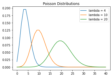
Now suppose that random variable $X$ describes the number of visitors per night, and that $P(X=n)$ denotes the probability of $n$ people visiting between 7 and 9 P.M. Let $\lambda$ denote the average number of visitors per night as the population parameter, and suppose that the P.D.F of $X$ is as follows: $P(X=x) = \frac{\lambda^x e^-\lambda}{x!}$ .

In such a case, $X$ is called the random variable of a Poisson distribution. In fact, such a random variable retains three key characteristics:

Independence

Consistency

Non-clusteredness

The first condition, independence, means that events in one time interval or space are independent from, and do not affect the probabilities of, events in other time intervals and spaces. The second condition, consistency, implies that the rate of the events’ occurrences is consistent. Finally, the third condition, non-clusteredness, signifies that the events must not be clustered together in a short timeframe.

The coffee shop example above is a rather oversimplified real-life example of where a Poisson distribution might be seen. In reality, a Poisson distribution is essentially a binomial distribution under special circumstances–the number of trials must approach infinity, and the probability of success must approach zero. In other words, if a binomial distribution describes the probability of observing $k$ successes among $n$ trials with $p$ as the probability of success,

$p(k) = {}_{n}C_{k} \cdot p^k \cdot (1-p)^{n-k},$

if $n \longrightarrow \infty \;\; \text{and}\;\; p \longrightarrow 0,$

then $P(X=k) = \frac{\lambda^k e^-\lambda}{k!}$ . The proof is shown below.

We start with the basic binomial distribution formula:

$p(x) = {}_{n}C_{x} \cdot p^x \cdot(1-p)^{n-x}$

In the case of Poisson distributions, $\lambda = np$ , and substituting $\lambda /n$ in place of $p$ yields:

$p(x) = {}_{n}C_{x} \cdot (\lambda/n)^x \cdot(1-\lambda/n)^{n-x}$

Then after manipulating the form thrice,

$p(x) = \frac{n!}{(n-x)! \cdot x!} \cdot (\lambda/n)^x \cdot(1-\lambda/n)^{n-x}$

$p(x) = \frac{n(n-1)(n-2) \cdot\cdot\cdot(n-x+1)}{x!} \cdot (\frac{\lambda^x}{n^x}) \cdot(1-\frac{\lambda}{n})^{n-x}$

$p(x) = \frac{n(n-1)(n-2) \cdot\cdot\cdot(n-x+1)}{n^x} \cdot (\frac{\lambda^x}{x!}) \cdot(1-\frac{\lambda}{n})^{n-x}$

As described above, take the limit of $p(x)$ as $n$ approaches infinity.

$\lim_{n \to \infty} p(x) = \lim_{n \to \infty} \frac{n(n-1)(n-2) \cdot\cdot\cdot(n-x+1)}{n^x} \cdot (\frac{\lambda^x}{x!}) \cdot(1-\frac{\lambda}{n})^{n}\cdot(1-\frac{\lambda}{n})^{-x}$

and since the first and last terms are equivalent to one,

$\lim_{n \to \infty} p(x) = \lim_{n \to \infty} (\frac{\lambda^x}{x!}) \cdot(1-\frac{\lambda}{n})^{n}$

$\lim_{n \to \infty} p(x) = \lim_{n \to \infty} (\frac{\lambda^x}{x!}) \cdot \left\{ (1-\frac{\lambda}{n})^{\frac{-n}{\lambda}} \right\}^{-\lambda} = \frac{\lambda^x \cdot e^{-\lambda}}{x!} \blacksquare$

Using the moment generating function, we can also find the mean and the standard deviation of a Poisson distribution.

$M(t) = \mathbb{E}[e^{tx}] = \sum_{x=0}^{\infty} e^{tx}p(x)$

$= \sum_{x=0}^{\infty} e^{tx} \cdot \frac{\lambda^xe^{-\lambda}}{x!} = e^{-\lambda} \cdot \sum_{x=0}^{\infty} \frac{(e^t \lambda)^x}{x!}$

Given the McLaurin series of $e^x$ ,

$e^x = \sum_{n=0}^{\infty} \frac{x^n}{n!}$

$e^{-\lambda} \cdot \sum_{x=0}^{\infty} \frac{(e^t \lambda)^x}{x!} = e^{-\lambda} \cdot e^{\lambda e^t} = e^{\lambda(e^t-1)}$

$\therefore M(t) = e^{\lambda(e^t-1)}$

The $k^{th}$ moment of random variable X is given by:

$\mu_k = \mathbb{E}(X^k)$

And the mean and median expressed in terms of moments are:

$\mu = \mathbb{E}(X) \;\;\;,\;\;\; \sigma = \mathbb{E}(X^2) - \mathbb{E}^2(X)$

$M(t) = \mathbb{E}[e^{tX}]$

When t=0, use McLaurin series of $e^x$

$M(t) = \mathbb{E}[e^{tX}] = \mathbb{E}\;[\sum_{k=0}^{\infty}\frac{(tX)^k}{k!}]$

$= \mathbb{E}[1 + tX + (tX)^2/2! + \cdot\cdot\cdot \;+ (tX)^k/k! + \cdot\cdot\cdot ]$

$= 1 + t\mathbb{E}(X) + t^2\mathbb{E}(X^2)/2! + \cdot\cdot\cdot \;+ t^k\mathbb{E}(X^k)/k! + \cdot \cdot \cdot$

$= 1+\mu_1 \cdot t \;+ \mu_2 \cdot t^2/2! + \cdot \cdot \cdot \; + \mu_k \cdot t^k/k! + \cdot \cdot \cdot$

Therefore, the $k^{th}$ derivative of $M(t)$ at $t=0$ is the $k^{th}$ moment.

$M^{k}(t) = \mathbb{E}[X^k], \;\;\;\; t=0$

Applying the above conclusion down below,

$\mu = \mathbb{E}(X) \;\;\;,\;\;\; \sigma^2 = \mathbb{E}(X^2) - \mathbb{E}^2(X)$

$\mu = M'(t) = [e^{\lambda(e^t-1)}]' = [e^{\lambda(e^t-1)}]\cdot (\lambda e^t), \;\;\;\; (t=0)$

$\therefore \; \mu = \lambda$

$\sigma^2 = M''(t) - (M'(t))^2 = [e^{\lambda(e^t-1)}]'' - \lambda^2, \;\;\;\; (t=0)$

With some basic algebra,

$\sigma^2 = \lambda, \;\;\; \sigma = \sqrt{\lambda}$

import matplotlib.pyplot as plt
import numpy as np
import math

x = np.linspace(-5, 5, 1000)
# y = 1 / (1 + np.e**(-x))
# mu = 0
# sigma = 1
# normal: y = 1 / (sigma * np.sqrt(2*np.pi)) * np.e**(-0.5*((x-mu)/sigma)**2)

lambdaP = 4
lambdaP2 = 10
lambdaP3 = 20

k = np.linspace(0, 40, 41) # k = np.ndarray
kList = list(k)
newK = list()

for i in kList:
  newK.append(math.factorial(int(i)))
# print(newK)
newKNP = np.asarray(newK)
# type(newKNP) # np.ndarray
 
y = (lambdaP**k) * (np.e**(-lambdaP)) / newKNP 
y2 = (lambdaP2**k) * (np.e**(-lambdaP2)) / newKNP 
y3 = (lambdaP3**k) * (np.e**(-lambdaP3)) / newKNP 

# type(y)
plt.plot(k.tolist(), y.tolist())
plt.plot(k.tolist(), y2.tolist())
plt.plot(k.tolist(), y3.tolist())

plt.legend(["lambda = 4", "lambda = 10", "lambda = 20"])
plt.title("Poisson Distributions")

# also works, but generates two separate plots
# fig, ax = plt.subplots()
# ax.plot(k,y)

# fig, ax2 = plt.subplots()
# ax2.plot(k,y2)
 

Poisson Distributions with Different Lambdas

The $\Gamma$ DistributionPermalink

The definition of a gamma function is as follows:

Definition

$\Gamma(x) = \int_0^\infty t^{x-1}e^{-t} dt$

With integration by parts, the second property can be proven in less than three lines. And by substituting one in place of $x$ , the third property can also be easily shown. With the second and third properties, the first one is then trivial.

Properties

$\Gamma(n) = (n-1)!$

$\Gamma(n+1) = n\Gamma(n)$

$\Gamma(1) = 1$

Gamma distribution PDF

Replace x by alpha, t by x from definition.

$\Gamma(\alpha) = \int_0^{\infty} x^{\alpha-1} \cdot e^{-x} dx$

$1 = \frac{1}{\Gamma(\alpha)} \cdot \int_0^{\infty} x^{\alpha-1}e^{-x} dx$

Substitute $x$ for $\beta \cdot y$

$\int_0^{\infty} x^{\alpha-1}e^{-x} dx = \int_{0}^{\infty} (\beta \cdot y)^{\alpha-1} \cdot e^{-\beta \cdot y} \cdot \beta \cdot dy$

$1 = \int_0^{\infty} \frac{1}{\Gamma(\alpha)} \cdot x^{\alpha-1}e^{-x} dx = \int_{0}^{\infty} \frac{\beta^\alpha}{\Gamma(\alpha)} \cdot y^{\alpha-1} e^{-\beta y} dy$

Replace $y$ by $x$ ,

$f(x | \alpha, \beta) = \frac{\beta^{\alpha}}{\Gamma(\alpha)} \cdot x^{\alpha-1} \cdot e^{-\beta x}, \;\;\;\;\; (x\geq0)$

$f(x | \alpha, \beta) = 0, \;\;\;\;\; (x<0)$

Mean, Variance of Gamma Distribution

$\lambda = \frac{\alpha}{\beta}, \;\;\;\;\; \sigma^2 = \frac{\alpha}{\beta^2}$

Proof:

We start with the momemt generating function:

$M(t) = \int_{0}^{\infty} \frac{\beta^{\alpha}}{\Gamma(\alpha)} \cdot x^{\alpha-1} \cdot e^{(t-\beta)x} dx$

Substitute $-\beta y = (t-\beta)x$

$M(t) = \int_{0}^{\infty} \frac{\beta^{\alpha}}{\Gamma(\alpha)} \cdot (\frac{\beta y}{\beta -t})^{\alpha-1} \cdot e^{-\beta y} \cdot (\frac{\beta}{\beta-t}) dy$

$= \frac{\beta^{\alpha}}{\Gamma(\alpha)} \int_{0}^{\infty} (\frac{\beta^{\alpha} \cdot y^{\alpha-1}} {(\beta -t)^{\alpha}}) \cdot e^{-\beta y} dy$

$= \frac{\beta^{\alpha}}{(\beta-t)^{\alpha}} \cdot \underbrace {\frac{1}{\Gamma(\alpha)} \cdot \int_{0}^{\infty} \beta^{\alpha} \cdot y^{\alpha-1} \cdot e^{-\beta y} \;dy}_{= 1}$

Since

$f(x | \alpha, \beta) := \frac{\beta^{\alpha}}{\Gamma(\alpha)} \cdot x^{\alpha-1} \cdot e^{-\beta x}, \;\;\;\;\; (x\geq0),$

$\int_{0}^{\infty} f(x | \alpha, \beta) \;dx = \int_{0}^{\infty}\frac{\beta^{\alpha}}{\Gamma(\alpha)} \cdot x^{\alpha-1} \cdot e^{-\beta x} dx = 1$

$\therefore \;M(t) = \frac{\beta^{\alpha}}{(\beta-t)^{\alpha}}$

The rest of the steps then become trivial.

$\; M'(t) = \frac{\alpha \cdot\beta^{\alpha}}{(\beta-t)^{\alpha+1}} = \frac{\alpha}{\beta}, \;\;\;\; (\text{with}\;\; t=0)$

$\; M''(t) = \frac{\alpha \cdot \beta^{\alpha} \cdot (\alpha+1)}{(\beta -t)^{\alpha+2}} = \frac{\alpha(\alpha+1)}{\beta^{2}}, \;\;\;\; (\text{with}\;\; t=0)$

$\therefore \;\; \lambda = \frac{\alpha}{\beta}, \;\;\;\;\; \sigma^2 = M''(0) - [M'(0)]^{2} = \frac{\alpha}{\beta^2}$

ConclusionPermalink

Distributions and statistical inferences based on those distributions are key in parametric statistics. In this post, I mainly went over Bernoulli, Poisson, and gamma distributions, although my intention was to go over several others. For binomial, multinomial, $\chi^2$ , and $\beta$ distributions, I will likely create a separate post on them. Although this blog post took longer to create than I had anticipated, I hope I learned much from the experience. Thanks for reading.

Twitter Facebook LinkedIn

Junhyung Park

Dive into Distributions

MotivationPermalink

Bernouille Trials, DistributionPermalink

Poisson DistributionPermalink

The $\Gamma$ DistributionPermalink

ConclusionPermalink

You May Also Enjoy

A Brief Look into Antidepressants

Thoughts on OCD (Obsessive-Compulsive Disorder)

Episode with Gastritis

Reflections Concerning Biomedical Research

Junhyung Park

MotivationPermalink

Bernouille Trials, DistributionPermalink

Poisson DistributionPermalink

The Γ\Gamma DistributionPermalink

ConclusionPermalink

You May Also Enjoy

A Brief Look into Antidepressants

Thoughts on OCD (Obsessive-Compulsive Disorder)

Episode with Gastritis

Reflections Concerning Biomedical Research

The $\Gamma$ DistributionPermalink