Distributions II

In this post, I discuss the gamma, chi-squared, and exponential distributions.

Background

Recently, I realized that I needed to refresh my memory of some important distributions that showed up in a Bayesian statistics book that I was studying. Those distributions included the gamma, the chi-squared, and the exponential distributions, and while I was brushing up on them, I decided to use the opportunity to record what I studied. (After all, there is no better way to study something than to explain it to someone else.) Given that I already posted on binomial and poisson distributions, this post will cover the three aforementioned distributions: their definitions, properties, and examples. The sources I referenced include: video by Lawrence Leemis on the gamma distribution, jbstatistics on chi-square distribution, this open-source textbook on exponential distributions from BCcampus Open Publishing, under CC BY 4.0.

---

Gamma Distribution

\[\begin{align} X \sim \Gamma(\alpha, \lambda) \end{align}\]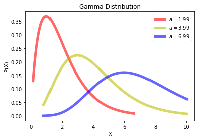

import numpy as np
import matplotlib.pyplot as plt
import scipy.stats as stats
import os
import seaborn as sns
from scipy.stats import gamma

def show_gamma():

    a1 = 1.99
    a2 = 3.99
    a3 = 6.99

    x1 = np.linspace(gamma.ppf(0.01, a1), gamma.ppf(0.99, a1), 100)
    x2 = np.linspace(gamma.ppf(0.01, a2), gamma.ppf(0.99, a2), 100)
    x3 = np.linspace(gamma.ppf(0.01, a2), gamma.ppf(0.99, a2), 100)

    plt.plot(x1, gamma.pdf(x1, a1), 'r', lw=5, alpha=0.6, label='$a={0}$'.format(a1))
    plt.plot(x2, gamma.pdf(x2, a2), 'y', lw=5, alpha=0.6, label='$a={0}$'.format(a2))
    plt.plot(x3, gamma.pdf(x3, a3), 'b', lw=5, alpha=0.6, label='$a={0}$'.format(a3))

    # Arbitrarily select 3 lambda values
    # lambdas = [1,4,10]
    
    # k = np.arange(20)       # generate x-values
    # markersize = 8
    # for par in lambdas:
    #     plt.plot(k, stats.poisson.pmf(k, par),  '*--', label='$\lambda={0}$'.format(par))
    
    # Format the plot
    plt.legend()
    plt.title('Gamma Distribution')
    plt.xlabel('X')
    plt.ylabel('P(X)')

show_gamma()

Probability density function

\[\begin{align} f(x) = \frac{\lambda^\alpha}{\Gamma(\alpha)} \cdot x^{\alpha-1} e^{\lambda x} \;\; (x \geq 0) \end{align} \tag{1}\]

Mean and Variance

\[\begin{align} \mu = E(X) = \frac{\alpha}{\lambda} \end{align} \tag{2}\] \[\begin{align} \sigma^2 = Var(X) = \frac{\alpha}{\lambda^2} \end{align} \tag{3}\]

Moment Generating Function

\[\begin{align} M_X(t) = \frac{1}{(1-\frac{t}{\lambda})^{\alpha}} \;\; (t < \lambda) \end{align} \tag{4}\]

---

Exponential Distribution

\[\begin{align} X \sim expo(\lambda) \end{align}\]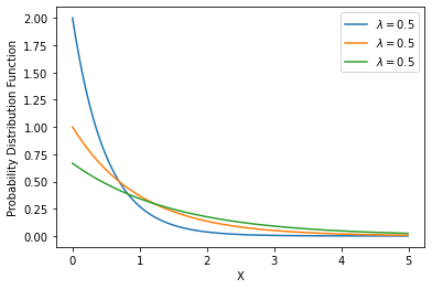

import numpy as np
import matplotlib.pyplot as plt
import scipy.stats as stats
import os
import seaborn as sns
from scipy.stats import gamma

def showExp():

    t = np.arange(0, 5, 0.01)
    
    plt.plot(t, stats.expon.pdf(t, 0, 0.5), label='$\lambda={}$'.format(0.5))
    plt.plot(t, stats.expon.pdf(t, 0, 1), label='$\lambda={}$'.format(0.5))
    plt.plot(t, stats.expon.pdf(t, 0, 1.5), label='$\lambda={}$'.format(0.5))

    plt.legend()
        
    plt.xlim(0,2)
    plt.xlabel('X')
    plt.ylabel('Probability Distribution Function')
    plt.axis('tight')
    plt.legend()

showExp()

Probability Distribution Function

\[\begin{align} f(x) = \left\{\begin{array}{ll} 1-e^{-\lambda x} & (\text {if } x \geq 0) \\ 0 & (\text {if } x < 0) \end{array}\right. \end{align} \tag{5}\]

Mean and Variance

\[\begin{align} \mu = E(X) = \frac{1}{\lambda} \end{align} \tag{6}\] \[\begin{align} \sigma ^ 2 = Var(X) = \frac{1}{\lambda ^ 2} \end{align} \tag{7}\]

Moment Generatng Function

\[\begin{align} M_X(t) = \frac{1}{(1-\frac{t}{\lambda})} \end{align} \tag{8}\]

---

Chi-squared Distribution

\[X \sim \chi^2(k)\]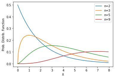

import numpy as np
import matplotlib.pyplot as plt
import scipy.stats as stats
import os
import seaborn as sns

def showChi2():

    t = np.arange(0, 8, 0.05)
    Chi2Vals = [1,2,3,5]
    
    # plt.plot(t, stats.chi2.pdf(t, 1), label='n={0}'.format(1))
    plt.plot(t, stats.chi2.pdf(t, 2), label='n={0}'.format(2))
    plt.plot(t, stats.chi2.pdf(t, 3), label='n={0}'.format(3))
    plt.plot(t, stats.chi2.pdf(t, 5), label='n={0}'.format(5))
    plt.plot(t, stats.chi2.pdf(t, 9), label='n={0}'.format(9))

    plt.legend()    
    plt.xlim(0,8)
    plt.xlabel('X')
    plt.ylabel('Prob. Distrib. Function')
    plt.axis('tight')

showChi2()

Probability Density Function

\[\begin{align} f(x) = \frac{1}{2^{k/2} \Gamma(k/2)} x^{\frac{k}{2} - 1} e^{-\frac{x}{2}} \end{align} \;\;\; \text{(k : shape parameter)} \tag{9}\]

Mean and Variance

\[\begin{align} \mu = E(X) = k \end{align} \tag{10}\] \[\begin{align} \sigma^2 = Var(X) = 2k \end{align} \tag{11}\]

Moment Generating Function

\[\begin{align} M_X(t) = (1-2t)^{-k/2} \end{align} \tag{12}\]

---

Conclusion

Whereas I covered basic information on some of the most widely-known distributions, I wish I could have dived more deeply into Bayesian statistics next time, since it serves as a cornerstone to many types of inferences and model evaluations in ML/DL projects. Anyways, this is the end of the post, and thansk for reading.