
Decision Tree
In this post, I will explain another popular supervised machine learning tool called a decision tree classifier.
Definition & Types
A decision tree classifier is a useful algorithm for classifying data. There are mainly two types of decision trees: classification trees and regression trees. The goal of a classification tree is to separate data into discrete classes. (For example, whether a select group of people have heart disease or not.) In a classification tree, a categorical question is used to separate data, and based on a true/false or yes/no answer, the data are classified into two groups.
Meanwhile, regression trees attempt to predict specific numerical values for provided data. (For example, the efficacy of a specific type of medicine, depending on how much of the medicine was administered (the dosage).) In other words, a regression tree possesses certain numerical threshold values that it uses to separate data into lower nodes, whereas a classification tree uses a series of true/false questions to split data. Regression trees can be particularly effective when a standard linear regression model fails to produce accurate numerical predictions, and especially when the data are grouped in a non-uniform manner depending on a specific variable.
Normally, when creating a decision tree, the topmost node is called the “root node,” and the nodes underneath are either called “internal nodes” or “leaf nodes,” If the data within those nodes can be separated into more nodes, then those nodes are called “internal nodes,” whereas if they cannot be separated, they are called “leaf nodes.”
In this post, I will focus on classification trees, which I found to be more intuitive and easier to understand, compared to regression trees.
Classification Trees
As stated above, a classification tree works by classifying data from a higher-tier node to two lower-tier nodes, based on a yes-or-no answer to a categorical question. But as with any classification algorithm, one can optimize the efficiency of the classification tree by asking the right questions first. Here, the “right” questions are the ones that can most efficiently separate the data into the desired categories.
To give a more concrete example, let’s assume that the task at hand is to separate 100 people into two categories: either with or without heart disease. The classification tree will first divide those 100 people into two categories, based on their yes-or-no answers to a root-node question. Although highly unlikely, if the root-node question manages to separate those 100 people perfectly based on whether they have heart disease or not, one could stop there–no need for more classification, after all.
Unfortunately, this ideal scenario doesn’t always conform to reality. In fact, it is natural to assume that no single question could perfectly filter out the desired group of people with/without heart disease. For example, suppose the root-node question is: “Do you drink more than five liters of alcohol per week?” Among those who answered positively, there may be a mix of people with and without heart disease. The same may hold true for those who answered negatively. In this case, the two internal nodes that result from the root-node question are called “impure,” which means that the nodes did not clearly discriminate based on the presence of heart disease.
Gini Impurity & Entropy
One can statistically measure the degree of impurity in two ways: Gini impurity index and entropy. The formula for the Gini impurity index is as follows:
\[I_G = 1-\sum_{i=1}^{n} p^2\]When data at a higher-tier node are separated into two lower-tier nodes, the $I_G$ value is calculated for each of the two lower-tier nodes. For this specific case, the square of the probability that a person may have heart disease, added to the square of the probability that a person may not have it, is the sum. The $I_G$ value is simply one minus that sum. Once the two $I_G$ values are calculated for both nodes, one has to find the total Gini impurity value, which is the weighted average of the two values.
The Gini impurity value measures the degree of impurity, and since we want the nodes to be as “pure” as possible, the most efficient tree can be created by asking the question with the lowest associated Gini impurity value. Once we reach the point where the total Gini impurity value no longer decreases, we finish the classification tree and make the lowest-tier nodes into leaf nodes.
There is another way to calculate impurity, which is by using the entropy equation. In chemistry, entropy is generally described as a measure of the state of disorderliness. In information theory, entropy is a measure of uncertainty. When we classify data into categories, uncertainty shrinks as we gain more information. In the case of heart disease, if we can perfectly separate people based on whether they have heart disease or not, the information gain would be one. Consequently, the resulting entropy would be zero. Therefore, the most efficient classification trees first use the questions that can most quickly reduce the entropy to zero.
The equation for entropy in information theory is as follows:
\[I_H = -\sum_{j=1}^{c} p_j \cdot log_2(p_j)\]Here, similar to how we calculated the Gini impurity value, the $p$ value either describes the probability of “yes” or “no” to the classification problem at hand. The only difference lies in the slightly different computation method, which for the entropy equation, involves calculating $p_j \cdot log_2(p_j)$ first.
Scikit-learn Implementation
The following code blocks are from one of StatQuests’ tutorials on decision trees. The used dataset is from the University of California Irvine’s Machine Learning Repository, and was originally provided by the Cleveland Clinic Foundation in 1988.
Importing Packages & Data
import pandas as pd
import numpy as np
import matplotlib.pyplot as plt
from sklearn.tree import DecisionTreeClassifier # imported to build a classification tree
from sklearn.tree import plot_tree
from sklearn.model_selection import train_test_split
from sklearn.model_selection import cross_val_score # imported to perform cross validation
from sklearn.metrics import confusion_matrix # imported to *create* a confusion matrix
from sklearn.metrics import plot_confusion_matrix # imported to *draw* a confusion matrix
df = pd.read_csv('processed.cleveland.csv', header=None)
df.head()
| 0 | 1 | 2 | 3 | 4 | 5 | 6 | 7 | 8 | 9 | 10 | 11 | 12 | 13 | |
|---|---|---|---|---|---|---|---|---|---|---|---|---|---|---|
| 0 | 63 | 1 | 1 | 145 | 233 | 1 | 2 | 150 | 0 | 2.3 | 3 | 0 | 6 | 0 |
| 1 | 67 | 1 | 4 | 160 | 286 | 0 | 2 | 108 | 1 | 1.5 | 2 | 3 | 3 | 2 |
| 2 | 67 | 1 | 4 | 120 | 229 | 0 | 2 | 129 | 1 | 2.6 | 2 | 2 | 7 | 1 |
| 3 | 37 | 1 | 3 | 130 | 250 | 0 | 0 | 187 | 0 | 3.5 | 3 | 0 | 3 | 0 |
| 4 | 41 | 0 | 2 | 130 | 204 | 0 | 2 | 172 | 0 | 1.4 | 1 | 0 | 3 | 0 |
df.columns = ['age', 'sex', 'cp', 'restbp', 'chol', 'fbs', 'restecg', 'thalach', 'exang', 'oldpeak', 'slope', 'ca', 'thal', 'hd']
# df.columns = ['parameter1', 'parameter2' [...] ] sets the column names to matching names.
df.head() # .head() prints the first 5 rows, including the column name
| age | sex | cp | restbp | chol | fbs | restecg | thalach | exang | oldpeak | slope | ca | thal | hd | |
|---|---|---|---|---|---|---|---|---|---|---|---|---|---|---|
| 0 | 63 | 1 | 1 | 145 | 233 | 1 | 2 | 150 | 0 | 2.3 | 3 | 0 | 6 | 0 |
| 1 | 67 | 1 | 4 | 160 | 286 | 0 | 2 | 108 | 1 | 1.5 | 2 | 3 | 3 | 2 |
| 2 | 67 | 1 | 4 | 120 | 229 | 0 | 2 | 129 | 1 | 2.6 | 2 | 2 | 7 | 1 |
| 3 | 37 | 1 | 3 | 130 | 250 | 0 | 0 | 187 | 0 | 3.5 | 3 | 0 | 3 | 0 |
| 4 | 41 | 0 | 2 | 130 | 204 | 0 | 2 | 172 | 0 | 1.4 | 1 | 0 | 3 | 0 |
Cleaning Data: Finding/Replacing Missing Values
df.dtypes # Identify the data type for the fourteen columns
age          int64
sex          int64
cp           int64
restbp       int64
chol         int64
fbs          int64
restecg      int64
thalach      int64
exang        int64
oldpeak    float64
slope        int64
ca          object
thal        object
hd           int64
dtype: object
The columns ca and thal, which are the number of blood vessels counted via fluoroscopy and the parameter corresponding to a thallium heart scan, respectively, have the object data type, which implies the existence of a mix of data types.
df['ca'].unique()
array(['0', '3', '2', '1', '?'], dtype=object)
df['thal'].unique()
array(['6', '3', '7', '?'], dtype=object)
The question mark, which most likely signifies missing data values, is present in both the ca and thal columns. To see exactly on which rows the question mark appears, the df.loc() method is used, which pinpoints the location in which the parameter value is true.
df.loc[(df['ca'] == '?') | (df['thal'] == '?')] # .loc() shows the location of the rows.
| age | sex | cp | restbp | chol | fbs | restecg | thalach | exang | oldpeak | slope | ca | thal | hd | |
|---|---|---|---|---|---|---|---|---|---|---|---|---|---|---|
| 87 | 53 | 0 | 3 | 128 | 216 | 0 | 2 | 115 | 0 | 0.0 | 1 | 0 | ? | 0 |
| 166 | 52 | 1 | 3 | 138 | 223 | 0 | 0 | 169 | 0 | 0.0 | 1 | ? | 3 | 0 |
| 192 | 43 | 1 | 4 | 132 | 247 | 1 | 2 | 143 | 1 | 0.1 | 2 | ? | 7 | 1 |
| 266 | 52 | 1 | 4 | 128 | 204 | 1 | 0 | 156 | 1 | 1.0 | 2 | 0 | ? | 2 |
| 287 | 58 | 1 | 2 | 125 | 220 | 0 | 0 | 144 | 0 | 0.4 | 2 | ? | 7 | 0 |
| 302 | 38 | 1 | 3 | 138 | 175 | 0 | 0 | 173 | 0 | 0.0 | 1 | ? | 3 | 0 |
df_new = df.loc[(df['ca'] != '?') & (df['thal'] != '?')]
df_new.head() # new DataFrame object with no missing values marked by question mark.
| age | sex | cp | restbp | chol | fbs | restecg | thalach | exang | oldpeak | slope | ca | thal | hd | |
|---|---|---|---|---|---|---|---|---|---|---|---|---|---|---|
| 0 | 63 | 1 | 1 | 145 | 233 | 1 | 2 | 150 | 0 | 2.3 | 3 | 0 | 6 | 0 |
| 1 | 67 | 1 | 4 | 160 | 286 | 0 | 2 | 108 | 1 | 1.5 | 2 | 3 | 3 | 2 |
| 2 | 67 | 1 | 4 | 120 | 229 | 0 | 2 | 129 | 1 | 2.6 | 2 | 2 | 7 | 1 |
| 3 | 37 | 1 | 3 | 130 | 250 | 0 | 0 | 187 | 0 | 3.5 | 3 | 0 | 3 | 0 |
| 4 | 41 | 0 | 2 | 130 | 204 | 0 | 2 | 172 | 0 | 1.4 | 1 | 0 | 3 | 0 |
One-Hot Encoding
To minimize the risk of unnecessarily jumbling up the data table, we must separate the table into two parts: the part that contains known classifications (y), and the part that contains data used to make predictions (x).
After this is done, we will use one-hot encoding to separate the columns whose values possess categorical meaning into several, independent columns with ones and zeros. The logic behind one-hot encoding is elaborated in more detail on the post about support vector machines, but the essence of one-hot encoding lies in treating categorical and quantitative data differently.
For example, the columns cp and slope are two of the seven columns that contain categorical data. As for the meaning behind the numerical values, he following information was retrieved alongside the data freely available from the repository.
cp: chest pain type
- Value 1: typical angina
- Value 2: atypical angina
- Value 3: non-anginal pain
- Value 4: asymptomatic
slope: the slope of the peak exercise ST segment
- Value 1: upsloping
- Value 2: flat
- Value 3: downsloping
X = df_new.drop('hd', axis=1).copy() # axis=1 implies dropping a column, not a row (axis=0)
y = df_new['hd'].copy()
X.head()
| age | sex | cp | restbp | chol | fbs | restecg | thalach | exang | oldpeak | slope | ca | thal | |
|---|---|---|---|---|---|---|---|---|---|---|---|---|---|
| 0 | 63 | 1 | 1 | 145 | 233 | 1 | 2 | 150 | 0 | 2.3 | 3 | 0 | 6 |
| 1 | 67 | 1 | 4 | 160 | 286 | 0 | 2 | 108 | 1 | 1.5 | 2 | 3 | 3 |
| 2 | 67 | 1 | 4 | 120 | 229 | 0 | 2 | 129 | 1 | 2.6 | 2 | 2 | 7 |
| 3 | 37 | 1 | 3 | 130 | 250 | 0 | 0 | 187 | 0 | 3.5 | 3 | 0 | 3 |
| 4 | 41 | 0 | 2 | 130 | 204 | 0 | 2 | 172 | 0 | 1.4 | 1 | 0 | 3 |
y.head()
0    0
1    2
2    1
3    0
4    0
Name: hd, dtype: int64
To perform one-hot encoding for only one column, we pass in the column name and the dataframe object as parameters to the get_dummies() function of the pandas library. For example, should we choose the column cp, which stands for ‘chest pain,’ we can split the column containing four values (1,2,3,4), into four columns containing either zero or one.
pd.get_dummies(X, columns=['cp']).head()
| age | sex | restbp | chol | fbs | restecg | thalach | exang | oldpeak | slope | ca | thal | cp_1 | cp_2 | cp_3 | cp_4 | |
|---|---|---|---|---|---|---|---|---|---|---|---|---|---|---|---|---|
| 0 | 63 | 1 | 145 | 233 | 1 | 2 | 150 | 0 | 2.3 | 3 | 0 | 6 | 1 | 0 | 0 | 0 |
| 1 | 67 | 1 | 160 | 286 | 0 | 2 | 108 | 1 | 1.5 | 2 | 3 | 3 | 0 | 0 | 0 | 1 |
| 2 | 67 | 1 | 120 | 229 | 0 | 2 | 129 | 1 | 2.6 | 2 | 2 | 7 | 0 | 0 | 0 | 1 |
| 3 | 37 | 1 | 130 | 250 | 0 | 0 | 187 | 0 | 3.5 | 3 | 0 | 3 | 0 | 0 | 1 | 0 |
| 4 | 41 | 0 | 130 | 204 | 0 | 2 | 172 | 0 | 1.4 | 1 | 0 | 3 | 0 | 1 | 0 | 0 |
As we can see, the column cp has been split into four independent columns: cp_1, cp_2, cp_3, and cp_4. Similarly, by using one-hot encoding, we need to split other columns as well, such as restecg, slope, ca, and thal.
X_encoded = pd.get_dummies(X, columns=['cp', 'restecg', 'slope', 'thal'])
X_encoded.head()
| age | sex | restbp | chol | fbs | thalach | exang | oldpeak | ca | cp_1 | ... | cp_4 | restecg_0 | restecg_1 | restecg_2 | slope_1 | slope_2 | slope_3 | thal_3 | thal_6 | thal_7 | |
|---|---|---|---|---|---|---|---|---|---|---|---|---|---|---|---|---|---|---|---|---|---|
| 0 | 63 | 1 | 145 | 233 | 1 | 150 | 0 | 2.3 | 0 | 1 | ... | 0 | 0 | 0 | 1 | 0 | 0 | 1 | 0 | 1 | 0 |
| 1 | 67 | 1 | 160 | 286 | 0 | 108 | 1 | 1.5 | 3 | 0 | ... | 1 | 0 | 0 | 1 | 0 | 1 | 0 | 1 | 0 | 0 |
| 2 | 67 | 1 | 120 | 229 | 0 | 129 | 1 | 2.6 | 2 | 0 | ... | 1 | 0 | 0 | 1 | 0 | 1 | 0 | 0 | 0 | 1 |
| 3 | 37 | 1 | 130 | 250 | 0 | 187 | 0 | 3.5 | 0 | 0 | ... | 0 | 1 | 0 | 0 | 0 | 0 | 1 | 1 | 0 | 0 |
| 4 | 41 | 0 | 130 | 204 | 0 | 172 | 0 | 1.4 | 0 | 0 | ... | 0 | 0 | 0 | 1 | 1 | 0 | 0 | 1 | 0 | 0 |
5 rows × 22 columns
Now that we have one-hot encoded values in the aforementioned four columns, we need to convert values in the y object (pandas.series.Series) to either zero or one. This is because our goal is binary classification based on whether someone has heart disease or not, using a classification tree. The current y object contains five values: 0, 2, 1, 3, 4, as seen from y.unique(), with numbers one, two, three, and four indicating various degrees of heart disease severity. Therefore, we will convert all numbers greater than or equal to one (1,2,3,4) into one, and leave the zero in place.
y.unique()
# type(y) returns pandas.core.series.Series
array([0, 2, 1, 3, 4], dtype=int64)
y.replace(to_replace=2, value=1, inplace=True)

y.replace(to_replace=3, value=1, inplace=True)
y.replace(to_replace=4, value=1, inplace=True)
y.unique()
array([0, 1], dtype=int64)
Building Decision Tree & Visualizing Results
Now that preprocessing the data is over, we need to use the DecisionTreeClassifier function to build the actual tree. To do that, we first perform a 70-30 split of data into training and test data. Then we use a 10-fold cross-validation method with GridSearchCV to find the best parameters for max_depth, min_samples_leaf and min_samples_split. In other words, when we split the data into ten folds, we randomly choose seven of them to be training data, and three of them to be test data. After repeating multiple trials with different permutations, the parameters that yield the best accuracy are chosen. The following information was taken from Scikit-learn’s website.
- max_depth: maximum depth of tree
- min_samples_split: the minimum number of samples to split a node
- min_samples_leaf: the minimum number of samples on a leaf node
The problem central to building accurate decision trees, however, still remains: overfitting the data. We say that we ‘overfit’ the data, when we overemphasize accuracy when training the model with the training data. Since the actual, unseen data may deviate from the training data, by attempting to build the ‘perfect’ model with training data, we may actually end up with a less accurate model–especially if the test data significantly deviate from the training data.
There are many ways to solve the problem, and this article from towards data science by Rukshan Pramoditha nicely summarizes various ways to resolve this issue. The StatQuest tutorial used the cost-complexity pruning method to find the optimum parameter value ccp_alpha, which essentially describes the degree to which the tree is pruned. Higher values for ccp_alpha imply more pruning.
Given the complexity of the process, I decided to instead use GridSearchCV to find the best parameter values for the three parameters specified above. The following code block is from the aforementioned website.
from sklearn.model_selection import GridSearchCV
import seaborn as sns
import matplotlib.pyplot as plt


X_train, X_test, y_train, y_test = train_test_split(X_encoded, y, random_state=42)
tree = DecisionTreeClassifier(random_state=42)
tree = tree.fit(X_train, y_train)

opt = {'max_depth': [2,3,4,6,8,10,12,15,20], 'min_samples_leaf': [1,2,4,6,8,10,20,30], 'min_samples_split': [1,2,3,4,5,6,8,10]}

grid = GridSearchCV(tree, param_grid=opt, scoring='accuracy', n_jobs=-1, cv=10, return_train_score=True)
grid.fit(X_train, y_train)
grid.best_estimator_.fit(X_train, y_train)


y_predict = grid.best_estimator_.predict(X_test)
y_true = y_test


print(grid.best_params_)
{'max_depth': 3, 'min_samples_leaf': 6, 'min_samples_split': 2}
Here, we see that the maximum tree depth is three, the minimum number of samples on a leaf node is six, and the minimum number of samples on a node for splitting is two.
In order to visualize the results, we use the sns.heatmap function.
matrix = confusion_matrix(y_true, y_predict)

y_labels = ['No HD', 'Has HD']
x_labels = ['No HD', 'Has HD']


sns.heatmap(matrix, annot=True, cmap='Blues', xticklabels=x_labels, yticklabels=y_labels)

plt.xlabel('Predicted')
plt.ylabel('True')
Text(33.0, 0.5, 'True')
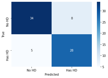
Here, we see that thirty-four out of fourty-two people with heart disease were correctly classified (80.95%), and among the thirty-three people without heart disease, twenty-eight were correctly classified (84.84%).
Conclusion
In this post, I explained the concepts of a decision tree, with specific focus on classification trees. Because I did not optimize the ccp_alpha parameter necessary for cost-complexity pruning, I could not visualize the tree using the plot_tree method, although I hope to use ccp_alpha optimization to solve the overfitting problem soon. Nonetheless, the result turned out to be fairly accurate, with over 80% of the test data correctly identified for both categories. This is the end of the post, and I hope you enjoyed reading.