
CNN with TensorFlow
In this post, I will cover my first attempt at learning about convolutional neural networks.
Convolutional Neural Networks
This blog post documents my first attempt at learning about convolutional neural networks, and is by no means a comprehensive guide on the topic. For more information, the following sources provide more detailed explanations.
- Blog post on CNN by Toward Data Science
- Similar post by Medium
- CNN cheatsheet by Stanford’s CS230
- François Chollet’s Deep Learning with Python.
Structure
The diagram below encapsulates the various design elements of a convolutional neural network, hereinafter referred to as simply “cnn.” This diagram, which was taken from a 2019 paper by Tabian, Fu, and Khodaei published on MDPI, is under the Creative Commons Attribution License, and the reference for the paper is provided below.
.PNG)
The inner workings of a cnn can be described as essentially a two-step process, with multiple layers in each of the steps. The two steps are feature learning and classification, with Conv2D and pooling layers in feature learning, and flatten, dense, and activation layers in classification.
- Feature Learning
- Convolution layer (Conv)
- Pooling layer
- Classification
- Flattening layer
- Fully connected layer (Dense)
- Activation layer
Convolution
The convolution step involves filling in the elements of an initial feature map using a filter (or kernel), considering the stride and the padding style in the process. Here, the depth of the filter must match the depth of the input image. For example, for the MNIST and Cats/Dogs datasets, the input depths are one and three, respectively, so the input depths for their filters must also be one and three. While studying the convolution step, I found more detailed explanations with excellent graphics at: Stanford CS230, this blog, and this article.
Activation function
After the convolution calculation, the ReLu activation function is used to convert elements of the initial feature map–that is, negatives are mapped to zero, and positives are mapped to themselves. This picture demonstrates how to apply ReLu to an initial feature map generated by a convolution layer, although copyright laws prohibit the picture’s display in this post.
As with other neural networks, the reason why an activation function is used is because of non-linearity. For a network to learn more complex patterns in the data, non-linearity must be introduced to the model. However, a neural network, at its basic framework, consists of many layers that pass on values to one another using two kinds of basic linear operations.
- Dot product between weight matrix and input vector
- Addition to bias vector
Since multiple linear operations can be expressed as a single linear operation, without any nonlinearity introduced to the model, having several layers produces no better performance than having just one layer. Adding a nonlinear activation function resolves this issue, as well as preventing node outputs from growing infinitely, which significantly slows down calculations. (For example, all outputs produced from the sigmoid function are between one and zero.)
Pooling
After applying ReLu to the initial feature map, use pooling methods to reduce the dimension of the feature map. Usually, the pooling method to use is maxpool, although average pooling is another option. Only after pooling can one use the feature map as an input for the next convolution layer.
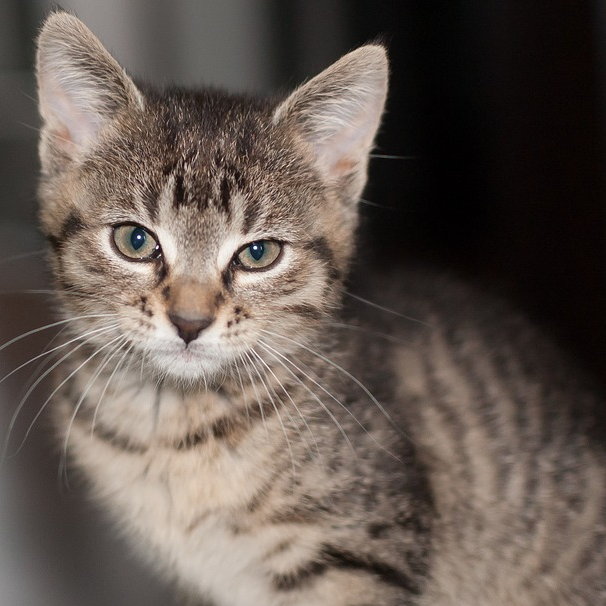
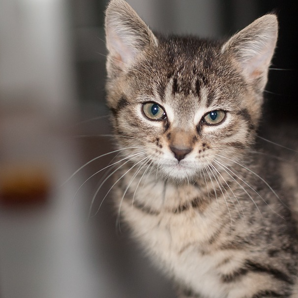
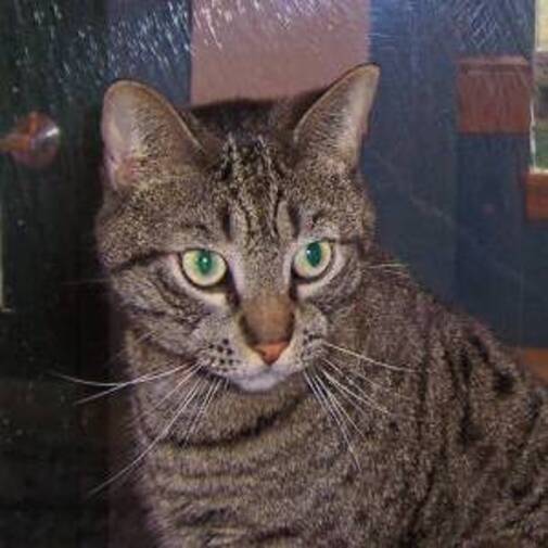
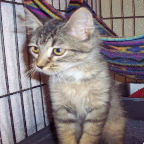
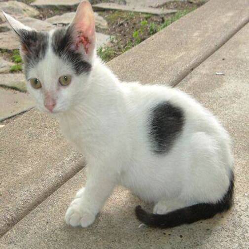
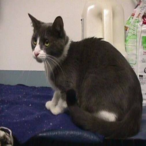
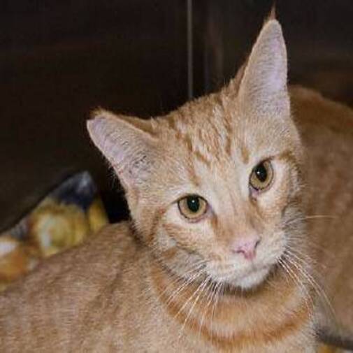
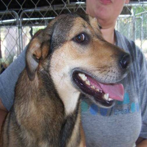
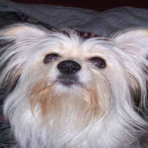
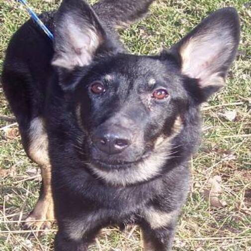
Pooling provides several benefits, including reducing overfitting and providing translation invariance. Translation invariance refers to classifying images with little regard to the spatial orientation of the object within an image. For example, the images below are of the same cat, but the cats are oriented differently. Nonetheless, pooling allows the model to correctly classify all four images as cats, since pooling reduces the difference between the feature maps of images with differently oriented objects. Pooling also helps with reducing overfitting, since it reduces the number of parameters.

Flattening
Flattening is essentially reducing the dimension of the pooling layer’s output, which is a three-dimensional tensor, or a stack of two-dimensional matrices. Since the Dense layer can only receive one-dimensional vectors as inputs, the flattening layer converts the 3D tensor output to the 1D vector input. This process is a lot easier to understand in terms of pictures than words, and this diagram does an excellent job demonstrating what the flattening layer does.
Dense layers & Activation layer
Since the task at hand is binary classification, the last layer should properly use the sigmoid activation function.
Cats vs Dogs
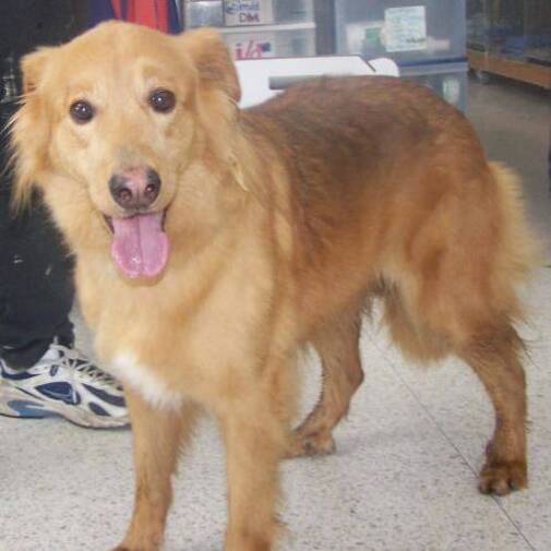
The code blocks below were borrowed from one of Tensorflow’s online tutorials on convolutional neural networks, which is under public domain via a Creative Commons license. The dataset import and the train-test-split steps are not shown below for brevity, but the 25,000 images in the dataset were split into train and test sets, with 22,500 and 2,500 images in each. In the 22,500 images belonging to the train set, there were 11,250 images of dogs and the same number of images for cats. Meanwhile, in the 2,500 images reserved for the test set, there were 1,250 images of cats, and the same number for dogs. The nine images below show some of the pictures in the dataset provided by Kaggle.
import os
import zipfile
import random
import tensorflow as tf
from tensorflow.keras.optimizers import RMSprop
from tensorflow.keras.preprocessing.image import ImageDataGenerator
from shutil import copyfile
print(len(os.listdir('/tmp/cats-v-dogs/training/cats/')))
print(len(os.listdir('/tmp/cats-v-dogs/training/dogs/')))
print(len(os.listdir('/tmp/cats-v-dogs/testing/cats/')))
print(len(os.listdir('/tmp/cats-v-dogs/testing/dogs/')))
11250
11250
1250
1250
model = tf.keras.models.Sequential([
    tf.keras.layers.Conv2D(16, (3, 3), activation='relu', input_shape=(150, 150, 3)),
    tf.keras.layers.MaxPooling2D(2, 2),
    tf.keras.layers.Conv2D(32, (3, 3), activation='relu'),
    tf.keras.layers.MaxPooling2D(2, 2),
    tf.keras.layers.Conv2D(64, (3, 3), activation='relu'),
    tf.keras.layers.MaxPooling2D(2, 2),
    tf.keras.layers.Flatten(),
    tf.keras.layers.Dense(512, activation='relu'),
    tf.keras.layers.Dense(1, activation='sigmoid')
])

model.compile(optimizer=RMSprop(lr=0.001), loss='binary_crossentropy', metrics=['acc'])
/usr/local/lib/python3.7/dist-packages/keras/optimizer_v2/optimizer_v2.py:356: UserWarning: The `lr` argument is deprecated, use `learning_rate` instead.
  "The `lr` argument is deprecated, use `learning_rate` instead.")
TRAINING_DIR = "/tmp/cats-v-dogs/training/"
train_datagen = ImageDataGenerator(rescale=1.0/255.)
train_generator = train_datagen.flow_from_directory(TRAINING_DIR,
                                                    batch_size=250,
                                                    class_mode='binary',
                                                    target_size=(150, 150))

VALIDATION_DIR = "/tmp/cats-v-dogs/testing/"
validation_datagen = ImageDataGenerator(rescale=1.0/255.)
validation_generator = validation_datagen.flow_from_directory(VALIDATION_DIR,
                                                              batch_size=250,
                                                              class_mode='binary',
                                                              target_size=(150, 150))
Found 22498 images belonging to 2 classes.
Found 2500 images belonging to 2 classes.
history = model.fit(train_generator, epochs=15, steps_per_epoch=90,
                    validation_data=validation_generator, validation_steps=6)
Epoch 1/15
5/90 [>.............................] - ETA: 58s - loss: 3.5931 - acc: 0.5120
90/90 [==============================] - 113s 917ms/step - loss: 0.8283 - acc: 0.5976 - val_loss: 0.5989 - val_acc: 0.6713
Epoch 2/15
90/90 [==============================] - 79s 877ms/step - loss: 0.5883 - acc: 0.6873 - val_loss: 0.5569 - val_acc: 0.7187
Epoch 3/15
90/90 [==============================] - 77s 858ms/step - loss: 0.5327 - acc: 0.7263 - val_loss: 0.5830 - val_acc: 0.7127
Epoch 4/15
90/90 [==============================] - 78s 865ms/step - loss: 0.4876 - acc: 0.7642 - val_loss: 0.5174 - val_acc: 0.7453
Epoch 5/15
90/90 [==============================] - 80s 889ms/step - loss: 0.4338 - acc: 0.7998 - val_loss: 0.4196 - val_acc: 0.8073
Epoch 6/15
90/90 [==============================] - 78s 871ms/step - loss: 0.3992 - acc: 0.8161 - val_loss: 0.3951 - val_acc: 0.8240
Epoch 7/15
90/90 [==============================] - 79s 872ms/step - loss: 0.3537 - acc: 0.8426 - val_loss: 0.4481 - val_acc: 0.8087
Epoch 8/15
90/90 [==============================] - 78s 869ms/step - loss: 0.3191 - acc: 0.8588 - val_loss: 0.5730 - val_acc: 0.7173
Epoch 9/15
90/90 [==============================] - 78s 860ms/step - loss: 0.2706 - acc: 0.8831 - val_loss: 0.4904 - val_acc: 0.7787
Epoch 10/15
90/90 [==============================] - 79s 873ms/step - loss: 0.2300 - acc: 0.9050 - val_loss: 0.7066 - val_acc: 0.7473
Epoch 11/15
90/90 [==============================] - 78s 869ms/step - loss: 0.1872 - acc: 0.9259 - val_loss: 0.5348 - val_acc: 0.7820
Epoch 12/15
90/90 [==============================] - 78s 863ms/step - loss: 0.1433 - acc: 0.9437 - val_loss: 0.5344 - val_acc: 0.8180
Epoch 13/15
90/90 [==============================] - 79s 872ms/step - loss: 0.1219 - acc: 0.9547 - val_loss: 0.5759 - val_acc: 0.8047
Epoch 14/15
90/90 [==============================] - 79s 880ms/step - loss: 0.0912 - acc: 0.9665 - val_loss: 0.6851 - val_acc: 0.8020
Epoch 15/15
90/90 [==============================] - 79s 878ms/step - loss: 0.0820 - acc: 0.9722 - val_loss: 0.6474 - val_acc: 0.8207
After fifteen epochs, the model achieved a 97.22% accuracy rate for the training set, while the number was slightly less for the validation set, at 82.07%. When the history object is plotted with matplotlib, there is clear indication of overfitting with validation loss peaking after about six epochs, so it would probably be best to stop after six epochs.
%matplotlib inline

import matplotlib.image  as mpimg
import matplotlib.pyplot as plt

#-----------------------------------------------------------
# Retrieve a list of list results on training and test data
# sets for each training epoch
#-----------------------------------------------------------
acc=history.history['acc']
val_acc=history.history['val_acc']
loss=history.history['loss']
val_loss=history.history['val_loss']

epochs=range(len(acc)) # Get number of epochs

#------------------------------------------------
# Plot training and validation accuracy per epoch
#------------------------------------------------
plt.plot(epochs, acc, 'r', "Training Accuracy")
plt.plot(epochs, val_acc, 'b', "Validation Accuracy")
plt.title('Training and validation accuracy')
plt.figure()

#------------------------------------------------
# Plot training and validation loss per epoch
#------------------------------------------------
plt.plot(epochs, loss, 'r', "Training Loss")
plt.plot(epochs, val_loss, 'b', "Validation Loss")
plt.figure()
.png)
.png)
References:
Tabian, I.; Fu, H.; Sharif Khodaei, Z. A Convolutional Neural Network for Impact Detection and Characterization of Complex Composite Structures. Sensors 2019, 19, 4933. https://doi.org/10.3390/s19224933